General linear models - Gaussian GLM (single categorical predictor)
This post was originally posted on my personal website on 18-07-2021. It has been updated as of 15-04-2023 to use Tidier.jl for data pre-processing
Session setup
As always, the first thing we need to do is download and load the required packages to perform these operations.
# Download required packages, if necessary (remove # to evaluate code)
# Pkg.add(["DataFrames", "CSV", "PalmerPenguins", "GLM", "Tidier.jl", "CairoMakie", "AlgebraOfGraphics", "GLM", "Effects"])

# Load required packages into current session
using DataFrames             # Create and manipulate DataFrame objects
using CSV                    # Import and process .csv files
using PalmerPenguins         # Access PalmerPenguins dataset
using GLM                    # Fit linear models
using Tidier                 # Tidyverse-like syntax for data manipulation
using CairoMakie             # Plotting utilities
using AlgebraOfGraphics      # Plotting utilities
using GLM                    # Fit linear models
using Effects                # Compute marginal means
Load data
The next step is to load the data we are going to analyse. We are going use the built-in Palmer penguins dataset (Gorman et al. 2014) that is made available through the PalmerPenguins.jl package (Horst et al. 2020). It contains body morphology measurements for 344 individual penguins from three species of penguins collected from three different islands in the Palmer Archpelago in Antarctica. There are 11 rows of data with missing data that we will remove from the dataset prior to analysis.
# Load PalmerPenguins data
df = DataFrame(PalmerPenguins.load(; raw = false))

# Drop the rows containing NA values
df = dropmissing(df, [:body_mass_g, :sex])
df = disallowmissing!(df)

# Show first 10 rows
first(df, 10)
10×7 DataFrame
Row │ species island bill_length_mm bill_depth_mm flipper_length_mm body_mass_g sex
│ String15 String15 Float64 Float64 Int64 Int64 String7
─────┼─────────────────────────────────────────────────────────────────────────────────────────────
1 │ Adelie Torgersen 39.1 18.7 181 3750 male
2 │ Adelie Torgersen 39.5 17.4 186 3800 female
3 │ Adelie Torgersen 40.3 18.0 195 3250 female
4 │ Adelie Torgersen 36.7 19.3 193 3450 female
5 │ Adelie Torgersen 39.3 20.6 190 3650 male
6 │ Adelie Torgersen 38.9 17.8 181 3625 female
7 │ Adelie Torgersen 39.2 19.6 195 4675 male
8 │ Adelie Torgersen 41.1 17.6 182 3200 female
9 │ Adelie Torgersen 38.6 21.2 191 3800 male
10 │ Adelie Torgersen 34.6 21.1 198 4400 maleResearch question
To illustrate how to fit and interpret a simple Gaussian GLM in Julia, we need to define our research question/hypothesis. Let's say that we are interested in whether the body mass (given as body_mass_g in df) of the three different penguins species is different. In other words, are one or more of the penguin species that were sampled either significantly lighter or heavier than the other species?
Exploratory data analysis
The first thing we should always be doing when analysing a new dataset is checking that the data is correct (e.g. there are no transcription errors, the data imported correctly, all the data is labelled correctly, ect...).
For example, one of the first things I always do is make sure that all the groups of interest are present in the dataset and the sample sizes are correct. We know from reading the help file for the Palmer penguins dataset that there should be three penguin species (Adelie, Gentoo and Chinstrap) and the total sample size across all penguins is n = 333.
# Count number of samples per penguin species
n_species = @chain df begin
    @group_by(species)
    @summarise(n = nrow())
end
3×2 DataFrame
Row │ species n
│ String15 Int64
─────┼──────────────────
1 │ Adelie 146
2 │ Chinstrap 68
3 │ Gentoo 119Brilliant. We have confirmed that the data was imported correctly - the data for all three penguin species are available, and we have confirmed that the sample sizes for the different penguin species are 146 (Adelie), 68 (Chinstrap) and 119 (Gentoo).
The next step is to visualise the data. Let's plot the distribution of body mass values for the three different penguin species. Below, we use the syntax :x => "x" to relabel each variable during the plotting procedure.
# Make boxplot of body mass by penguin species
data(df) *
    # Provide the column names to plot on the x and y axis
    mapping(
        :species => "Species",
        :body_mass_g => "Body mass (g)") *
    # Colour the bars by 'species'
    mapping(color = :species => "Species") *
    # Draw a boxplot
    visual(BoxPlot) |>
    # Make the final figure
    draw;
It looks like the median body mass (indicated by the bold black line in the middle of the boxes) is quite a bit higher for Gentoo penguins than either Adelie or Chinstrap penguins. Indeed, Gentoo penguins appear to weigh just over 1000g more than the other two species. The variance (i.e. spread of body mass values along the y-axis) appears to be relatively similar between the three penguin species.
Model fitting
Fitting a GLM is relatively simple in Julia. All we need to do is tell it what is our response variable (the response variable is the measurement we are interested in). Here, the response variable is (body_mass_g). We then specify our predictor variables to the right-hand side of this weird ~ (tilde) symbol. Our predictor variables are things we have recorded that we believe could be affecting the response variable. Here, our predictor variable was species. By fitting this model, we are testing the hypothesis that the body mass measurements taken from the 333 penguins in this study vary between the three penguin species. Thereafter, we need to tell Julia where these data are stored (df), and that we want a Gaussian GLM (Normal()), with an identity link function (GLM.IdentityLink).
The last argument we specify is contrast, which allows us to mainly specify the comparisons between categorical variables that we want to make. In this example, we are comparing measurements between Gentoo vs Adelie vs Chinstrap penguins, so we need to specify that we want effects coding. Effects coding will test whether each penguin species is different to the mean body mass across the other two penguin species. This is in contrast to treatment coding, which would compare each penguin species to the reference level. This will become more important when we build more complex models in later blog posts (e.g. including interaction terms). I won't go into detail here, other than to point you towards a great introduction to effects coding that you can read in the meanwhile.
# Fit Gaussian GLM
m1 = fit(
         # We want a GLM
         GeneralizedLinearModel,
         # Specify the model formula
         @formula(body_mass_g ~ 1 + species),
         # Where is the data stored?
         df,
         # Which statistical distribution should we fit?
         Normal(),
         # Which link function should be applied?
         GLM.IdentityLink(),
         # Specify effects coding (more on this in later posts)
         contrasts = Dict(:species => EffectsCoding()));
Let's inspect the model output.
# Print summary output
print(m1)
StatsModels.TableRegressionModel{GeneralizedLinearModel{GLM.GlmResp{Vector{Float64}, Normal{Float64}, IdentityLink}, GLM.DensePredChol{Float64, LinearAlgebra.CholeskyPivoted{Float64, Matrix{Float64}, Vector{Int64}}}}, Matrix{Float64}}
body_mass_g ~ 1 + species
Coefficients:
────────────────────────────────────────────────────────────────────────────────
Coef. Std. Error z Pr(>|z|) Lower 95% Upper 95%
────────────────────────────────────────────────────────────────────────────────
(Intercept) 4177.23 26.5856 157.12 <1e-99 4125.12 4229.34
species: Chinstrap -444.142 41.8047 -10.62 <1e-25 -526.077 -362.206
species: Gentoo 915.207 36.0772 25.37 <1e-99 844.497 985.917
────────────────────────────────────────────────────────────────────────────────Here, we get a table of the model coefficients. Let's break it down step-by-step:
The first thing to notice is that one of the species is missing from the table (
Adelieis missing from the table). Why?Well, the reason is that
Adeliepenguins are being used as the reference level to compare the other two species with.Let's take a look at the
Coef.column, as this is where most of the interesting information exists.Interpreting the
(Intercept): When we specify a Gaussian GLM with a categorical predictor as we have done here (remember that penguinspecieswas our predictor variable), the coefficient for the(Intercept)row is actually the mean value of the response variable (body_mass_g) for the missing level of the predictor. In other words, the(Intercept)coefficient represents the mean body mass (in grams) ofAdeliepenguins. So, the mean body mass forAdeliepenguins = 4177 grams (or 4.17kg).Interpreting categorical predictor variable coefficients: As above, when we specify a Gaussian GLM with a categorical predictor as we have done here (remember that penguin
specieswas our predictor variable), the coefficients for the levels of the predictor variable are the difference in the response variable (body_mass_g) to the reference level.E.g. The coefficient for
Chinstrappenguins = -444.14, which means that the mean body mass ofChinstrappenguins is 444.14 grams less thanAdeliepenguins (the reference level).Similarly, the coefficient for
Gentoopenguins = 915.21, which means that the mean body mass ofGentoopenguins is 915.21 grams more thanAdeliepenguins (the reference level).
This is all good and well, but we don't yet know if the mean body mass was statistically significantly different between the three penguin species.
Model inference
Now to the bit of the analysis that most ecologists are most interested in (at least to appease their reviewers: assessing statistical significance and calculating p-values). Here, we perform statistical inference, which basically means we are going to evaluate "which [model] coefficients are non-zero beyond a reasonable doubt, implying meaningful associations between covariates and the response?" Tredennick et al. 2021.
To do this, we will use a Likelihood Ratio Test (LRT). The LRT allows us to compare a model of interest with a null model that lacks some feature of the model of interest. For example, below we will compare our model of interest (containing the species predictor variable) with a null model which lacks the species predictor. This way we can ask whether adding information about species improved the likelihood of the data in comparison to the null model. Please see Tredennick et al. 2021 for an excellent introduction to using the LRT for model inference.
Below, we define our null model as model containing only a random-intercept only, which is probably the most common null model for basic statistical inference in ecology. The random intercept term in this model effectively represents random chance alone. In other words, this model formula represents the hypothesis that penguin body mass is not significantly different between the three species (i.e. a null hypothesis).
# Define null model to assess effect of 'species` on penguin body mass
# - Fit a random intercept only (indicated by y ~ 1)
mnull = fit(
         GeneralizedLinearModel,
         @formula(body_mass_g ~ 1),
         df,
         Normal(),
         GLM.IdentityLink());
And finally, we can perform a LRT to test that hypothesis that penguin body mass differed between the three penguin species sampled.
# Perform LRT
StatsModels.lrtest(mnull, m1)
Likelihood-ratio test: 2 models fitted on 333 observations
───────────────────────────────────────────────────────────────
DOF ΔDOF LogLik Deviance Chisq p(>Chisq)
───────────────────────────────────────────────────────────────
[1] 2 -2700.1455 215259665.9159
[2] 4 2 -2513.2729 70069446.8027 373.7453 <1e-81
───────────────────────────────────────────────────────────────The LRT tells us that including penguin species as a predictor significantly improved the fit of our model to the data relative to the null model (\(\chi\)2 = 373.75, d.f. = 2, P < 0.001). The LRT supports our alternative hypothesis that penguin body masses were different between the three penguin species sampled.
Marginal effects
Regression models, such as the GLM, can be very difficult to interpret and understand. For example, the distinction between treatment versus effects coding can make interpretations quite tricky, while the absence of one of the levels of the predictor variable (i.e. the reference level) is very confusing.
To get around this issue, we can calculate marginal effects (and uncertainty) to make understanding the model outputs easy and efficient. With a single categorical variable in our fitted GLM, the interpretation of the model results is about as straightforward as it will ever be. When the models get more complex (e.g. adding multiple predictors, mixing categorical and numeric predictors, adding interaction terms), the model outputs get more and more difficult.
Let's calculate the estimated marginal effects from our fitted model using the marvelous Effects.jl package. To do this, we need to specify which variable to calculate the effects over, which is going to be the penguin species column and store this information in a variable called design. Thereafter, we pass the design variable and the fitted GLM model (which we stored in m1) to the effects function to calculate the marginal effects.
# Calculate marginal effects
design = Dict(:species => unique(df.species))
eff_species = Effects.effects(design, m1)
3×5 DataFrame
Row │ species body_mass_g err lower upper
│ String15 Float64 Float64 Float64 Float64
─────┼───────────────────────────────────────────────────
1 │ Adelie 3706.16 38.1356 3668.03 3744.3
2 │ Gentoo 5092.44 42.241 5050.2 5134.68
3 │ Chinstrap 3733.09 55.8796 3677.21 3788.97The body_mass_g column contains the estimated marginal mean of the body mass of the three different penguin species, and the err column contains the standard error of the estimated marginal means (hereafter s.e.). The lower and upper columns contain the estimated marginal means \(\pm\) 1 s.e..
Ideally, we will usually want to report and visualise the estimated marginal means \(\pm\) a 95% confidence interval of the mean (which is 1.96 \(\pm\) s.e.). Below, we will calculate 1.96 \(\pm\) s.e. for each penguin species and store this value in the existing err column, and manually calculate the 95% confidence intervals (stored in lower_ci and upper_ci).
# Calculate 95% confidence interval of the mean marginal effect
eff_species_ci = @chain eff_species begin
    @group_by(species)
    @summarise(
        body_mass_g = body_mass_g,
        err = 1.96 * err,
        lower_ci = body_mass_g - err,
        upper_ci = body_mass_g + err
        )
end
3×5 DataFrame
Row │ species body_mass_g err lower_ci upper_ci
│ String15 Float64 Float64 Float64 Float64
─────┼──────────────────────────────────────────────────────
1 │ Adelie 3706.16 74.7458 3668.03 3744.3
2 │ Chinstrap 3733.09 109.524 3677.21 3788.97
3 │ Gentoo 5092.44 82.7923 5050.2 5134.68We can also make a plot of the estimated marginal means (and 95% confidence intervals) to quickly visualise the differences in body mass between penguin species.
# Plot mean and 95% CI of marginal effect
plt = data(eff_species_ci) *
        mapping(
            # Plot axes and create new labels for each axis
            :species => "Species",
            :body_mass_g => "Body mass (g)"
            ) *
        (visual(Scatter) + mapping(:err) * visual(Errorbars)) |>
        draw
FigureGrid()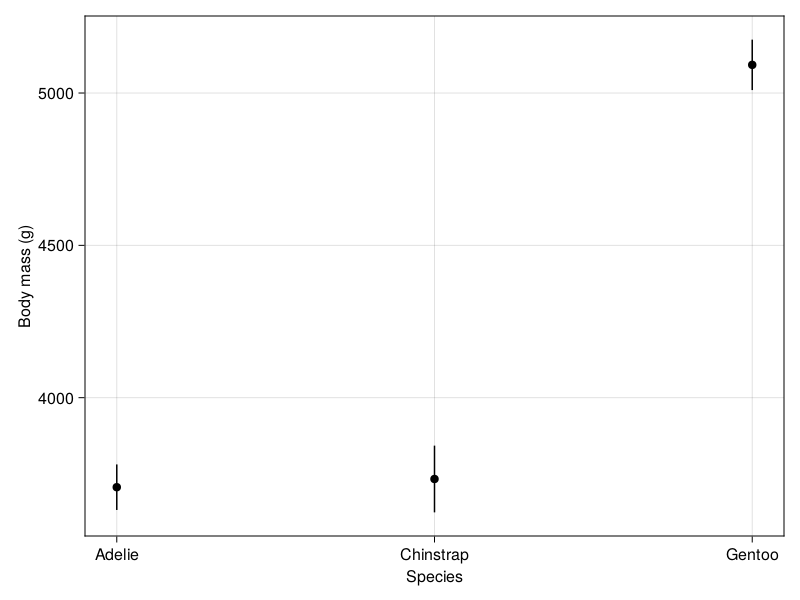
The plot clearly shows us that the average body mass of Gentoo penguins is significantly higher than both Adelie and Chinstrap penguins. On average, Gentoo penguins weigh more than 1200g (1.2kg) more than both Adelie (3706g) and Chinstrap penguins (3733g).
On the other hand, we can see that the body mass of Adelie and Chinstrap penguins are quite similar - the difference in the mean estimated body mass is only about 27 g. The overlapping 95% confidence intervals of the marginal means for these two penguin species is a pretty good indicator that there is no statistically significant difference in the body mass measurements.
Conclusion
In conclusion, we have completed a simple but thorough ecological data analysis using a Gaussian GLM using Julia. Due to the presence of a single categorical predictor in our model, this analysis can is roughly equivalent to a one-way analysis of variance (ANOVA), albeit we used a LRT not F-test, to calculate statistical significance. In the next few blogposts, we will work through progressively more complex examples of a Gaussian GLM (e.g. with numeric predictor variables, with combinations of numeric and categorical predictors, interaction terms, ect...). One aspect that we did not cover in this blogpost is evaluating the model fit using residual diagnostics (e.g. qqplot, residual vs fitted plots), which is an essential step in the model fitting workflow. This will be the topic of an upcoming blogpost - stay tuned!